1
2
3
4
5
6
7
8
9
10
11
12
13
14
15
16
17
18
19
20
21
22
23
24
25
26
27
28
29
30
31
32
33
34
35
36
37
38
39
40
41
42
43
44
45
46
47
48
49
50
51
52
53
54
55
56
57
58
59
60
61
62
63
64
65
66
67
68
69
70
71
72
73
74
75
76
77
78
79
80
81
82
83
84
85
86
87
88
89
90
91
92
93
94
95
96
97
98
99
100
101
102
103
104
105
106
107
108
| #include "Image_FFT.h"
void FFT_Shift(double * src,int size_w,int size_h){
for(int j=0;j<size_h;j++)
for(int i=0;i<size_w;i++){
if((i+j)%2)
src[j*size_w+i]=-src[j*size_w+i];
}
}
void ImageFFT(IplImage * src,Complex * dst){
if(src->depth!=IPL_DEPTH_8U)
exit(0);
int width=src->width;
int height=src->height;
double *image_data=(double*)malloc(sizeof(double)*width*height);
for(int j=0;j<height;j++)
for(int i=0;i<width;i++){
image_data[j*width+i]=GETPIX(src, j, i);
}
FFT_Shift(image_data,width, height);
FFT2D(image_data, dst, width, height);
free(image_data);
}
void Nomalsize(double *src,double *dst,int size_w,int size_h){
double max=0.0,min=DBL_MAX;
for(int i=0;i<size_w*size_h;i++){
max=src[i]>max?src[i]:max;
min=src[i]<min?src[i]:min;
}
double step=255.0/(max-min);
for(int i=0;i<size_w*size_h;i++){
dst[i]=(src[i]-min)*step;
dst[i]*=45.9*log((double)(1+dst[i]));
}
}
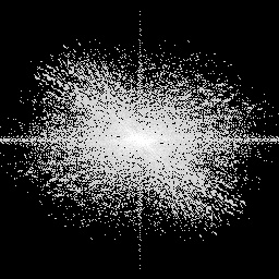
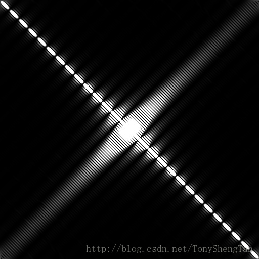
void getAmplitudespectrum(Complex * src,int size_w,int size_h,IplImage *dst){
double *despe=(double *)malloc(sizeof(double)*size_w*size_h);
if(despe==NULL)
exit(0);
double real=0.0;
double imagin=0.0;
for(int j=0;j<size_h;j++)
for(int i=0;i<size_w;i++){
real=src[j*size_w+i].real;
imagin=src[j*size_w+i].imagin;
despe[j*size_w+i]=sqrt(real*real+imagin*imagin);
}
Nomalsize(despe, despe, size_w, size_h);
for(int j=0;j<size_h;j++)
for(int i=0;i<size_w;i++){
cvSetReal2D(dst, j, i, despe[j*size_w+i]);
}
free(despe);
}
void ImageIFFT(Complex *src,IplImage *dst,int size_w,int size_h){
Complex *temp_c=(Complex*)malloc(sizeof(Complex)*size_w*size_h);
if(temp_c==NULL)
exit(0);
for(int i=0;i<size_w*size_h;i++)
Copy_Complex(&src[i],&temp_c[i]);
Complex *temp=(Complex*)malloc(sizeof(Complex)*size_w*size_h);
if(temp==NULL)
exit(0);
double *temp_d=(double *)malloc(sizeof(double)*size_w*size_h);
if(temp_d==NULL)
exit(0);
IFFT2D(temp_c,temp,size_w,size_h);
for(int j=0;j<size_h;j++)
for(int i=0;i<size_w;i++){
temp_d[j*size_w+i]=temp[j*size_w+i].real;
}
FFT_Shift(temp_d, size_w, size_h);
for(int j=0;j<size_h;j++)
for(int i=0;i<size_w;i++){
cvSetReal2D(dst, j, i, temp_d[j*size_w+i]);
}
free(temp);
free(temp_c);
free(temp_d);
}
|